COSC/MATH 146
Numerical Analysis Assignment 3, Newton's Method
Problem statement:
Newton's Method (AKA Newton-Raphson iteration) is one way used
to find zeros or roots of a function.
Using the method we are to compute the following:
- Find Sqrt (a) by solving x^2 - a = 0, for a = 5
- sin^3 (x) - exp (-a * x) = 0, for a = 0.1
- 2 * x - tan (x) = 0
- sqrt ( abs (x)) = 0
- exp(-x) = 0
Description of the algorithm
In implementing Newton's Method, we must consider a graph
of a function f where there is a definite slope at each
point and therefore exists a unique tangent line. If we continue
with that idea, at a certain point (x0,
f(x0)) on the graph of f
there is a tangent, which is a good approximation to the curve
around that point. This implies:
l(x) = f'(x0)(x-x0)
+ f(x0)
Hence the zero of l is an approximation to the zero
of f therefore:
x1 = x0
- [ f(x0) / f'(x0)]
Furthermore, starting with point x0,
we will continue and pass x1 obtained
from the proceeding formula. This process is then iterated to
produce a sequence of points. Under favorable conditions the
sequence of points will eventually approach a zero of f
which intersects the x-axis at a certain point. Newton's Method
can be summarized as the following:
xn+1 = xn -
[f(xn) / f'(xn)]
The program used for the assignment was not coded by me. I
found a much better one on the Internet with many more options
than I could have implemented. The Newton Method applet in which
I used were written by Professor Richard E. Williamson and can
be found here:
http://www.dartmouth.edu/~rewn/newton.html
Convergence Tests
The main convergence test I used was taken from an example
from the textbook where an output of a set of values for n,
xn, and f(xn)
were printed out. When the convergence starts happening, the
values of xn in the function starts to
eventually "repeat." This is when you can approximate
the root(s) of the function.
Another convergence test I used was complementary of the author
of the Java applet. He included a plotting option for the function.
Therefore I can somewhat estimate where the function converges
by looking at about where the graph of f starts approaching
the x-axis.
x^2 - a = 0, for a = 5
The roots found in this equation was -2.23606 and +2.23606.
By looking at the equation we know that it is going to be a
parabola pointing upward therefore can exists at most only 2
roots and they should both be equal and opposite to one another
because the trough is on the y = -5 axis. The starting values
chosen for the function was 1 and -1 because the function was
not so complicated and the roots should be somewhere near the
origin.
figure 1.1 By entering
the functions and the derivative of the function we get:

figure1.2 The plot of x^2 - 5= 0
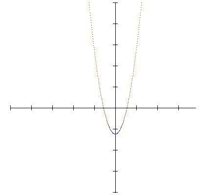
As we can see from the plot there
exists two roots.
Figure 1.3 the table of
outputs for the function
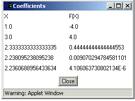
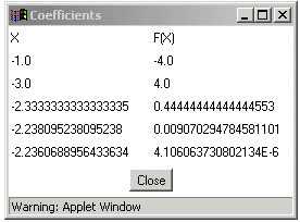
From the outputs of xn
and f(xn) we can see that the two
roots are -2.2360 and +2.2360. The convergence
was around +/- 2.23 and the rate was actually pretty fast. That
can possibly lead us to assume that perhaps the answer is not
so reliable. However, further verification with Maple assures
us with the roots of -2.236067977 and +2.236067977 for the function.
This matches about 5 digits of precision after the decimal point.
From this function we can conclude that the convergence
rate for it is fast. Also we now know that parabolas can only
have a maximum of 2 roots.
sin^3 (x) - exp (-a * x) = 0, for a = 0.1
Upon first locking at the function I knew that
it would be some sort of wave function but not exactly sure
what. The strange thing about this function is that I can't
seem to figure out what is going on. When I first entered the
function at a starting value of 1, that same value root is given
back with only one iteration. When I try another start value
for instance 2, 4, or 20, those same numbers are given back
as roots along with only 1 iteration. So then I plotted the
function and this is what I got:
figure 2.1 (x = -1-10, y
= -1 - 10)
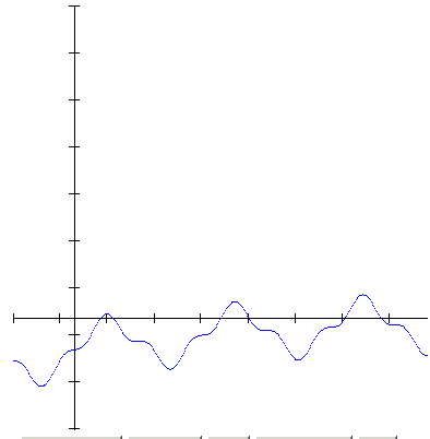
Figure 2.2 Strange function,
I changed the ranges and the new plot is ( x = -10-100, y =
-10-100)
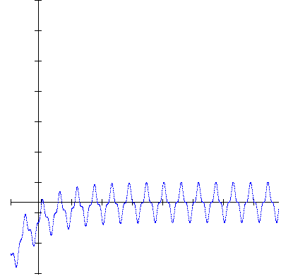
The function looks like it slowly evens out after
it passes the y-axis. So since the Java program does not give
good roots for the function, I decided to use the TI-85. Upon
plotting the function, I received a similar graph except for
the fact that the larger the value of x is, the period of the
wave gets smaller and smaller. The only few roots that I can
obtained from tracing on the calculator are 1.2698, 1.9345,
2.0337, 2.3809, 2.4063. If I had continue
on finding more roots, it appears that the values will become
more dense per x-increment units therefore leading me to believe
there exist an infinite number of roots.
I believe this is why whenever I pick a starting
value for the program, that exact same value is the root. The
roots are so bunched up per x-unit that there are so many roots
between each interval and any starting value I pick for the
program is right by a root.
Along with that, since the values of the roots
are so small and close in values, the graph given by the program
isn't necessarily correct. The graph in figure 2.2 looks like
it repeats itself over and over again after a certain x-value,
but that is wrong. It repeats itself because the computer can
not hold enough digits in memory so it has to truncate values
of x. That's why they appear to be the same period. However
if we plot the function on the calculator, we will see that
the period of the function gets smaller and smaller the larger
the x-value gets.
The convergence of the function is kind of hard
to tell. There was not really enough outputs to conclude anything
and also because the computer's precision was there lack of
in this function.
The accuracy of my first few digits were obtained
from the calculator and not the program. Even though I traced
to estimate the values of the roots, I believe they are much
more preferable compared to the root values the program computed.
I can conclude from this function that you must
be really careful how you enter the function into the computer.
Even thought the program gave me no warning, I entered the function
incorrectly and didn't realized it until I graphed it out on
the calculator. Most importantly, I learned that you can't always
believe the outputs of the computer of only one program. You
must verify it with another source.
2 * x - tan (x) = 0
The roots found in this function were -1.16556,
and +1.16556. The starting values of these roots were
1 and -1. They were chosen based on the form of the function
which included a tangent telling us that there will be a repeating
function. Also the values were chosen because they surround
the origin of 0 which is most often a root of many functions.
Figure 3.1 the function
entered
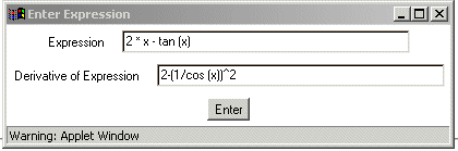
Figure 3.2 & 3.3
the roots found from the program
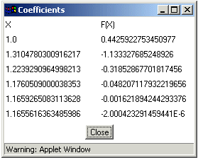
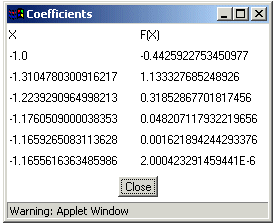
Figure 3.4 the plot of the
function
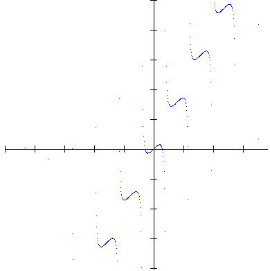
Figure 3.5 a closer look at the function
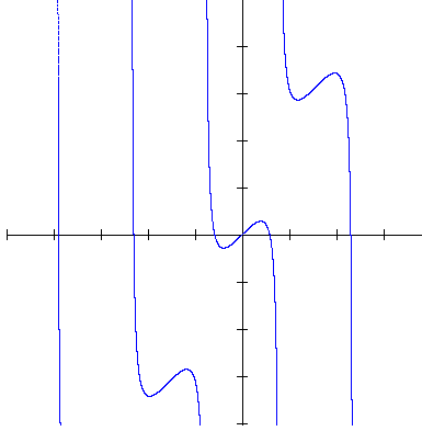
Figure 3.6 another look
at the function with a new range
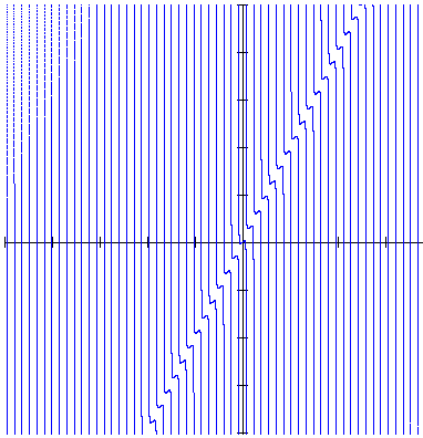
It appears according to the graphs that there are only 2 roots
(3 including 0). This explains why you get bizzare values when
enter a start value greater than 2 and less than -2. Those are
supposingly undefined.
We can observe from figures 3.2 and 3.3 that the function rapidly
converges, nearly doubling after each iteration.
I believe my answers for this function is pretty accurate up
to the computer max precision. These values can be verified
with the tracing on the calculator.
I can conclude from this function that trig-functions are pretty
tricky. It is extremely helpful if you are able to graph out
trig functions to guide you along your process.
sqrt ( abs (x)) = 0
The only root for this function is 0. It was a little
tricky finding the root because I started off with the values
of 1 and -1 again and the program could not find any roots.
Then I realized that one must root is zero because of the square
root operation. I had to set the start value to 0.001 and the
step to a samll value too to find this root in the program.
Figure 4.1 the function
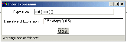
Figure 4.2 the root
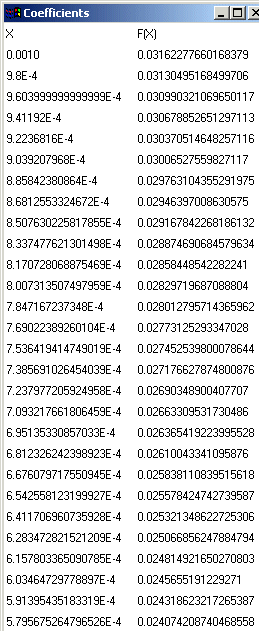
As we can see from figure 4.2 that root converges
quite slow, very abnormal for a Newton Method. We can also see
that the value approaching zero for xn
is also really slow too.
figure 4.3 the function
plot, we can see there do exist a root
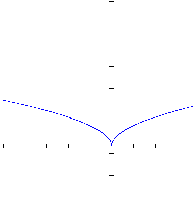
I believe my answer for this function is right
on, that is it is exactly 0. I verified it with by graphing
it out on the calculator and by solving for it on paper.
I can conclude from this function that the root(s)
somtimes can be right under your nose without you knowing it.
Like my professor said, "A little mathematics beats a lot
of computing anyday." If you think it through, it is more
obvious than you expect.
exp(-x) = 0
The programs outputs values incrementing by 1(or
the step value) from the starting value you entered and the
function gets smaller and smaller but never reaches zero.
Figure 5.1 function table
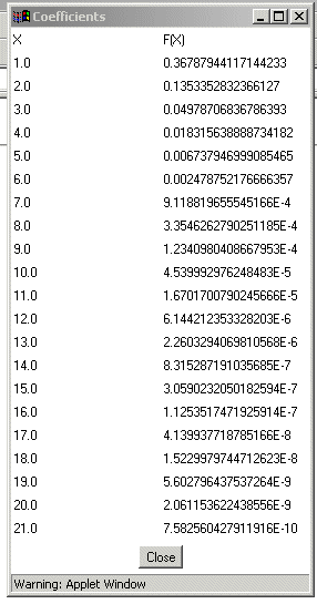
Figure 5.2 function graph
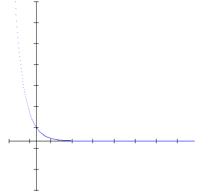
Well we know that an exponential function goes
to infinity so that's enough said. no need to find / compute
anything on the computer.
References
Cheney, Kincaid (1999). Numerical Mathematics
and Computing 4th Ed., Cole Publishing company.
Corliss,G. 2001. NumericalAnalysis Entry Page
[Online] http://studsys.mscs.mu.edu/~georgec/146.2001/
Professor Richard Williamson, Interactive Math
Programs [Online] http://www.dartmouth.edu/~rewn/newton.html
Appendix
A zip of the appendix can be downloaded here 


